5. DISTRIBUTION OF MEASUREMENTS
5.1 INTRODUCTION
Up to this point, the discussion has treated the "scatter" of measurements in an intuitive way, without inquiring into the nature of the scatter. This chapter will explore some of the methods for accurately describing the nature of measurement distributions. In practice, one must deal with a finite set of values, so the nature of their distribution is never known precisely. As always, one proceeds on the basis of reasonable assumptions.
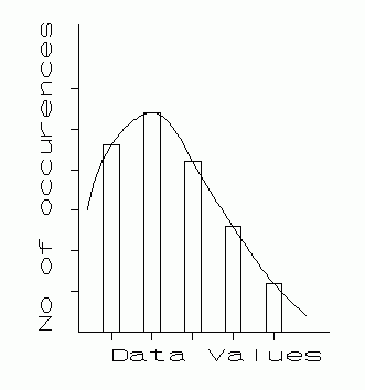
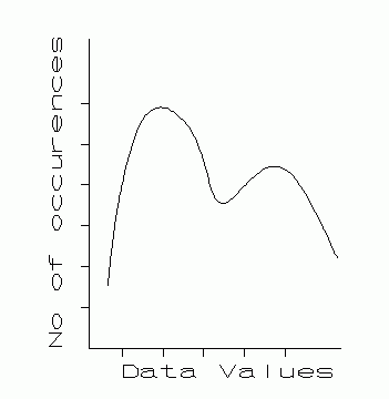
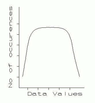
Consider a large number of repeated measured values of a physical quantity. Suppose the number of values is very large, and a bar graph (Fig. 5.1) is made of the number of occurrences of each value. The tops of the bars are connected with a smooth curve. Such a curve is called an error distribution curve. Such curves come in an infinite variety of shapes, as the four examples in Fig. 5.1 illustrate.
 |
 |
| Bar graph representation of an error distribution. |
A bimodal distribution. |
|---|
 |
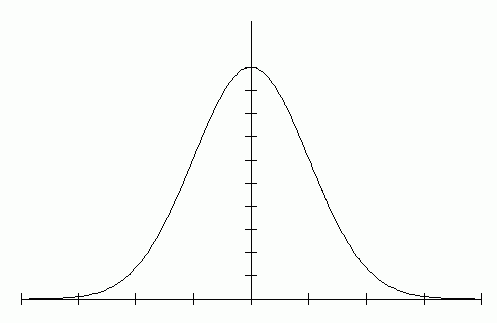 |
| A distribution with a flattened top. | Gaussian (normal) distribution very accurately drawn from computer generated data. |
|---|
One can often guess the shape of the curve, even with a finite set of values, especially such features as symmetry and spread. Just as we represent a set of values by one value (some kind of average), so also we can represent the shape of the distribution curves by measures of dispersion (spread), skewness, etc. We can describe the measurement and its uncertainty by just a few numbers. The mathematical discipline of statistics has developed systematic ways to do this.
5.2 MEASURES OF CENTRAL TENDENCY OF DATA
Some of the "measures of central tendency" commonly used are listed here for reference:
ARITHMETIC MEAN. (or simply the MEAN, or the AVERAGE): The sum of the measurements divided by the number of measurements.
GEOMETRIC MEAN. The nth root of the product of n positive measurements.
HARMONIC MEAN. The reciprocal of the average of the reciprocals of the measurements.
MEDIAN. The middle value of a set of measurements ranked in numerical order.
MODE The most frequent value in a set of measurements. (more precisely: the value at which the peak of the distribution curve occurs.)
5.3 MEASURES OF DISPERSION OF DATA
The difference between a measurement and the mean of its distribution is called the DEVIATION (or VARIATION) of that measurement. Measures of dispersion are defined in terms of the deviations. Some commonly used measures of dispersion are listed for reference:
AVERAGE DEVIATION FROM THE MEAN. (usually just AVERAGE DEVIATION, abbreviated lower case, a. d.): The average of the absolute values of the deviations.
| [5-1] |
 |
MEAN SQUARE DEVIATION. The average of the sum of the squares of the deviations.
| [5-2] |
 |
ROOT MEAN SQUARE DEVIATION The square root of the average of the squares of the deviations. Or, simply the square root of the mean square deviation.
| [5.3] |
 |
5.4 DISPERSION MEASURES APPROPRIATE TO GAUSSIAN DISTRIBUTIONS
The distributions encountered in physics often have a mathematical shape given by
| [5-4] |
 |
where x is a measurement, <x> is the mean, and f(x) is the ordinate of the distribution curve for that value of x. σ is the standard deviation. Distributions which conform to this equation are called Gaussian, or normal distributions. Fig. 5.4 has been accurately drawn to illustrate this curve. The shape of the Gaussian shows it to be symmetric about its highest value, and this highest value occurs at <x>.
The Gaussian distribution is so common that much of the terminology of statistics and error analysis has been built upon it. Furthermore, when one must deal with an unknown distri- bution, it is usually assumed to be Gaussian until contrary evidence is found.
The total width, or spread, of the Gaussian curve is infinite, as the equation shows. But Gaussians do differ in how much f(x) decreases for a given value of (x - <x>). Physicists sometimes define the "width" of such peaked curves by the "width at half height." This is measured by finding two points x1 and x2 such that f(x1) = f(x2) = f(<x>)/2. Then the "width at half height" is (x2 - x1). This is not very useful in statistical studies.
Statisticians have devised better measures of "width" of Gaussian curves by specifying a range of values of x which include a specified fraction of the measurements. Some are listed here:
STANDARD DEVIATION (or STANDARD ERROR, σ): A range within one standard deviation on either side of the mean will include approximately 68% of the data values. (This is not a definition.) A range within two standard deviations will include 95% of the data values.
PROBABLE ERROR (P.E.) (Definition) A range within one probable error on either side of the mean will include 50% of the data values. This is 0.6745σ.
RELIABLE ERROR (Def.) A range within one reliable error on either side of the mean will include 90% of the data values. This is 1.6949σ.
5.5 ESTIMATES OF DISPERSION OF THE "PARENT" DISTRIBUTION
The dispersion measures listed in the last section described the dispersion of the data sample. Had we taken more data, we would expect slightly different answers; both the mean and the dispersion depends on the size of the sample.
Ideally we want huge samples, for the larger the sample, the more nearly the sample mean approaches the "true" value. In statistical theory one speaks of the parent distribution, an infinite set of measurements of which our finite sample is but a subset. We must always be content with a finite sample, but we would like to use it to estimate the dispersion of the parent distribution. Statistical theory provides a simple way to do this:
| [5-5] |
 |
When this factor is applied to the root mean square deviation, the result is simply to replace n by (n-1). This new expression is called the
| [5-6] |
 |
Note that Eqs. 5.3 and 5.6 become more nearly identical as n gets large. The distinction between the two is mainly important for small samples.
Mathematical statistics texts may be consulted for an explanation of equation 5.5. Also see the books by Topping, Parratt, Beers, Barford, and Pugh-Winslow. The replacement of n by (n-1) us called Bessel's correction. A plausibility argument reveals the need for the correction, so we state it briefly here:
First, the case of n=1 can be eliminated form consideration; we can only average two or more quantities. When n = 2 the mean will lie halfway between the two values and both will have the same magnitude of deviation (but opposite signs). These two magnitudes are not independent. In fact, the number of independent deviations we get from n measurements is (n-1). So, when averaging the squared deviations, divide by the quantity (n-1), not n.
When samples are small, the spread of values will likely be less than that of a larger sample. The (n-1) "corrects" for this small-sample effect, giving a more realistic estimate of the spread of the parent distribution.
Quite a number of books presenting error analysis for the undergraduate laboratory ignore Bessel's correction entirely. There is some practical justification for this.
The difference between n and (n-1) is only 2% when n = 50. As n gets larger, the difference becomes less. So, when "enough" measurements are made, the difference matters little.
When very few measurements are made, the error estimates themselves will be of low precision. It can be shown, using careful and correct mathematical techniques, that the uncertainty of an error estimate made from n pieces of data is
| [5-7] |
100/√[2(n-1)]
So we'd have to average 50 independent values to obtain a 10% error in the determination of the error. We would need 5000 measurements to get an error estimate good to 1%. If only 10 measurements were made, the uncertainty in the standard deviation is 33%. This is why we have continually stressed that error estimates of 1 or 2 significant figures are sufficient when data samples are small.
This is one reason why the use of the standard deviation in elementary laboratory is seldom justified. How often does one take more than a few measurements of each quantity? Does one even take enough measurements to determine the nature of the error distribution? Is it Gaussian, or something else? One usually doesn't know. If it isn't close to Gaussian, the whole apparatus of the usual statistical error rules for standard deviation must be modified. But the rules for maximum error, limits of error, and avarage error are sufficiently conservative and robust that they can still be relibably used even for small samples. However, when three or more different quantities contribute to a result, a more realistic measure of error is obtained by using the `adding in quadrature' method described at the beginning of this section.
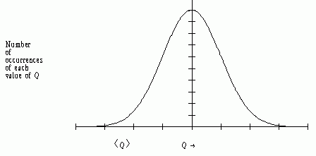 |
| Fig. 5.2. The Norman Curve (Gaussian). Measured values of Q are on the horizontal axis. <Q> is the mean value of Q. The marks along the horizontal axis are one standard deviation apart. |
|---|
5.6 ERRORS OF THE MEAN
All of the measures of dispersion or "width" introduced above express how far individual measurements deviate from the "true" mean. But we are usually more interested in the accuracy of the mean itself.
In chapter 3 we considered this problem, concluding that the error in an average was the error in each measurement divided by the square root of the number of measurements. This result expresses our confidence in any one isolated measurement. This is one of three commonly used measures of confidence in the mean; we list them here for completeness.
AVERAGE DEVIATION OF THE MEAN (Abbreviated upper case, A. D. M.) The average deviation divided by the square root of the number of measurements.
STANDARD DEVIATION OF THE MEAN (σm or σ<Q>) The standard deviation divided by the square root of the number of measurements.
PROBABLE ERROR OF THE MEAN (P. E. M.) The probable error divided by the square root of the number of measurements.
To illustrate the meaning of these, consider a set of, say, 100 measurements, distributed like Fig. 5.2. These should be sufficient to make a rough sketch of the shape of the curve, determine the mean, and calculate a standard deviation. Now suppose we took 10,000 measurements. Would the shape of the curve change much? Probably not. We would be able to sketch the curve with more precision, but its width and the value of the mean would change very little. Yet, with more measurements we are "more certain" of our calculated mean. The error measurements of the mean reflect this certainty, while the measures of dispersion describe the spread of individual measurements from the mean.
Also, with more data, the calculation of the measures of dispersion improves. Imagine the set of 10,000 measurements made up of 1000 sets of 10 measurements. From each set of 10 we calculate a mean. If we now look at these 1000 calculated means, they too form a distribution. If the data were Gaussian, this distribution of means will also be Gaussian. But this distribution of means will have a smaller width than the width of the data distribution itself. The standard deviation of the mean is smaller than the standard deviation of the measurements, by the factor 1/√n.
To carry this example further, if we calculate the standard deviation of the measurements in each sample of 10, we will get 1000 different values of standard deviation. These too form a distribution. It is shown, in more advanced treatments that the standard deviation of a standard deviation is
| [5-8] |
 |
where σ is the standard deviation of the measurements, and n is the number of measurements.
In scientific papers it is important to specify which measure of error is being used, and how many measurements were taken. Only then can readers properly interpret the quality of the results.
5.7 EFFICIENT CALCULATION OF THE STANDARD DEVIATION
The root-mean-square deviation and standard deviation definitions (Eqs. 5.2 and 5.6) are given in intuitively meaningful forms. But these equations are not in a form suitable for efficient calculation. We can easily derive an equation better suited to numerical computation.
In the following derivation all summations are from i=1 to i=n.
The standard deviation is defined by
| [5-9] |
 |
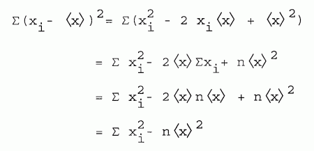 |
So:
| [5-10] |
 |
Many electronic calculators have a built-in routine which allows you to enter the xi values in succession. When this is done, the calculator has accumulated the sum of those values in one memory register, the sum of the squares of the values in another register, and may even have counted the entries and stored n in a register. These stored values are then easily recalled to calculate the standard deviation.
A similar procedure can be used for the rms deviation.
5.8 EXERCISES: (Starred exercises require calculus)
(8.1)* What percent of the measurements fall within the width at half height of a Gaussian curve?
(8.2) A set of measurements of a quantity is
878     849     804     755
816     833     781     735
964     795     817     807
862     801     778     810
778     799     819     797
Find the means, average deviations, and standard deviations for (1) each of the four groups, and (2) the whole group of twenty.
(8.3) Graph the distribution of problem 2. Note that a bar graph showing occurrences of each value would not be very informative, for few values occur more than once. It is better to graph the number of occurrences within a few ranges of values, as a teacher might display test scores.
5.9 FOOTNOTE TO CHAPTER 5
This chapter has been included for three reasons: (1) to introduce the statistical measures of error needed in the following chapter, (2) to provide a reference list of commonly encountered measures of error, and related terminology, and (3) to explain the important distinction between measures of dispersion of the data, and errors of the mean.
It is not expected that the student should memorize this material; it is included here as a reference source, to be used as needed.
The definitions given here (and throughout this lab manual) are consistent with current usage in physics, mathematical statistics and engineering. The student may (and should) confirm this by consulting the error analysis books given in the bibliography, other lab manuals in physics, and copies of current physics journals. The journals are the best source of examples of accepted practice in methods of reporting errors. The editors of the good journals insist that authors not be sloppy in these matters. But do not take as your guide the popular, general interest publications, such as Popular Science, news magazines, or the daily paper. Such publications are shamefully negligent in these matters, with the result that scientific facts are often presented in a most misleading manner. These are primarily sources of bad examples.
Chemistry, biology, earth sciences, astronomy, and even social sciences will be found to adhere to careful standards in reporting errors in their journals. Unfortunately, instructors in elementary courses often take a more cavalier attitude, seemingly unaware of current practice and current terminology used in research papers. If the student has any doubts about correct style, he should check up-to-date books and journal articles in his discipline.
Standards and styles were different even as recently as a few decades ago. For example, in the 1950's one frequently found mention of the "probable error" as a measure of uncertainty. Today, one seldom sees that term, the standard deviation is preferred instead. We list both in the table on the next page, to aid those who may read the older literature.
The relations between probable error and standard deviation are summarized below, and are only valid for Gaussian distributions.
Conversion factors, for Gaussian distributions only:
average deviation/standard deviation = 0.7979
standard deviation/average deviation = 1.2533
probable error/standard deviation = 0.6745
probable error/average deviation = 0.8453
probable error/average error = 0.8453
average error/probable error = 1.183
probable error/standard deviation = 0.6745
standard deviation/probable error = 1.4826
© 1999, 2004 by Donald E. Simanek.