USING LOGRARITHMIC GRAPH PAPER

Logarithmic graph paper is seldom seen by students in elementary courses. There seems to be a general impression that (1) it is too difficult to deal with, or (2) students "can pick it up" without instructions. Niether is true, in my opinion.

In the days of slide rules, students had (or ought to have had) intimate familiarity with logrithms and logarithmic scales, for every slide rule had at least two such scales. Nowadays many of these gory details are hidden in the innards of an electronic calculator or computer, a "black box" that grinds out numbers, whether or not those numbers have any significance.

Graphs with logarithmic scales are found in research papers and textbooks. One example is the usual graph of the electromagnetic spectrum. If students are to interpret such graphs intelligently, they need to directly experience the process of making one.

All sorts of computer graphing software is available. The most used software is designed for the needs of business, not science. Many such software packages simply cannot do the things necessary for dealing with the needs of physics.

7.8 LOGARITHMIC GRAPH PAPER

Logarithmic graph papers are available in many types. They simplify the process of linearizing exponential and power relations and determining the constants in their equation.

Fig. 7.8. Relabeling a logarithmic scale.

Examine the logarithmic scales of such paper. Typically the logarithmic scales come with partially labeled divisions. A sample is shown in Fig. 7.8.

Starting from the left, we see labels from 1 to 10, repeated three times. Each segment labeled from 1 to 10 is called a cycle. This sample has 3 cycles. The labeling already printed on the paper is for convenience only; the user must relabel the axes to suit the data.

For example, suppose you want to plot data values ranging from 2 units to 800 units on this three cycle log scale. The first cycle is labeled "as is" from 1 to 9. The second cycle is relabeled 10, 20, 30, 40, 50, 60, 70, 80, and 90. The third cycle is relabeled 100, 200, etc. to 1000.

Each cycle covers a range of values spanning one factor of 10. The next cycle covers a range 10 times larger, etc. The value zero does not appear on a logarithmic scale, for as x → 0, log (x) → -∞.

The "generic" labeling is done differently on different brands of paper. Some label the start of a cycle with "1"; some use "10". Some mark 1.5 and 2.5; some don't.

The user has less freedom in labeling a log scale than a linear one. The scales are directed, i.e., one-way, and cannot be labeled in the opposite direction.

The underlying principle of the log scale is that lengths along the scale are proportional to the logarithms of the plotted values. The C and D scales of slide rules are constructed the same way.

The user must carefully examine the markings of the scale to correctly interpret its subdivisions. Some intervals have 10 subdivisions, some only five (every second one of the ten being shown). Errors in the use of log paper result from failure to notice these differences in the way subdivisions are labeled.

Graph papers with one linear and one logarithmic scale are called semi-logarithmic, log-linear, or simply logarithmic. Graph papers with both scales logarithmic are called log-log, full log, or dual logarithmic.

As is evident from the 10 divisions of each cycle, these logarithmic scales represent base-10 logarithms.

EXPONENTIAL RELATIONS of the form

[7-12]

y = Ae^βx

where A and β are constant, can be rendered as straight lines on semi-log paper. To see this, take the logarithm of both sides of

[7-13]

^βx

which gives

[7-14]

log y - log A = x β log e = x β (0.43420...)

Plot x on the linear axis and y on the logarithmic axis. The resulting straight line will have slope

[7-15]

log y₂ - log y₁ ——————————————— = β log e x₂ - x₁

from which the constant β may be easily determined.

The y-intercept of the graph will be the value of the constant A.

The slope of a line on logarithmic paper must be interpreted with care. It may be evaluated in either of two ways.

(1) Choose two well-separated points on the line (x₁, y₁) and (x₂, y₂). Use these to evaluate the left side of equation (7-15).

(2) The value of the numerator of equation (7-15) may be found by length measurements on the graph, since the logarithms are proportional to lengths. Measure the length of one cycle on the paper. Measure the length between y₂ and y₁. Then

[7-16]

L/C = log_₂y - log_₁y

where L is the length along the log axis between the two points, and C is the length of one cycle measured along that axis.

This is true because for one cycle,

[7-17]

log (10y) - log (y) = log (10) = 1.

This method makes it unnecessary to look up or evaluate the logarithms of the data points.

Fig. 7.9. Semi-logarithmic
graph paper.

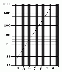
Example: This original graph (Fig 7.9) had cycles 4.15 cm long. On your computer screen, or the printed page, it will appear a different size. The variable x is plotted on the horizontal axis and y is plotted on the vertical axis. [Ignore the uneven spacing in the vertical lines. It is a fault of my diagram, which I intend to fix one of these days.]

When x = 0, then y = Ae⁰ = A. So the y-intercept is the value of A. But x = 0 lies off the edge of the graph, so this would not be a good way to find the value of A in this case. Let us postpone this problem and first find the slope.

Choose two points on the line. I chose the points with values x=2 and x=7 on the horizontal axis. Mark these points on your copy of Fig. 7.8. They have values of y=20 and y=500 on the vertical axis. A ruler shows that 20 and 500 are separated by 5.85 cm vertically.

The slope of the line is

[7-18]

5.85 cm ——————— 4.15 cm 1.41 ——————— = ————— = 0.2819 = β log e 7 - 2 5

and therefore, since log(e) = 0.4342945

[7-19]

 
    0.2819
α = —————— = 0.6491
    0.4343

The numerator on the left of Eq. 7-18 is dimensionless, so the units of β will be the reciprocal of the units of x.

Now we can evaluate the constant A. Take any value of x that is on the graph, say x = 7. From the graph, this gives y = 500. Then

[7-20]


     y    500   500
A = ——— = ——— = ————— = 5.317
     βx    7β   94.04
    e     e

So finally, the equation that represents this curve is

[7-21]

y = 5.317e^(0.6491)x

Notice that in this whole process we never had to take a logarithm of any data values.

EXERCISE (7.8) Check Eq. 7-21 by evaluating y for x = 3.4 and comparing the result with the graph. {Answer 48.32; the agreement is good.}

EXERCISE (7.9) Use Eq. 7-21 to calculate y for x = 6.2. Compare with the graph.

POWER RELATIONS of the form

[7-22]

y = Kx^p

may be rendered straight by plotting on log-log paper. Take the logarithm of both sides

[7-23]

log y = log K + p log x

Now if y is plotted against x on log-log paper we get a line of slope

[7-24]

log y₂ - log y₁ ——————————————— = p log x₂ - log x₁

where, as before, the points 1 and 2 are well-separated points on the straight line. Neither intercept has any special, useful, meaning on this graph! (On log paper log x never has a zero value.)

We have several ways to calculate the slope, once we have specified two well- separated points on the line, and obtained equation (7-24).

(1) Evaluate equation (7-24) by explicit calculation of the logarithms.

(2) Set up the right triangle and measure the lengths of the legs. Then, as before:

[7-25]

length of the "y" leg ——————————————————————— length of one "y" cycle —————————————————————————————— = p length of the "x" leg ——————————————————————— length of one "x" cycle

On most log-log graph paper, the lengths of the cycles on the x and y axes are simply related. If they are equal, then the slope is simply

[7-26]

length of one "y" leg ————————————————————— = tan q = p length of the "x" leg

So in this special case one may simply measure the angle, q, to determine the slope.

Fig. 7.10. Log-log graph paper.

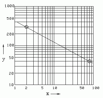
Example: Data that plots as a straight line on log-log paper can always be expressed by the relation

[7-27]

y = Kx^p

The constants K and p are to be determined from the graph. Two points have been chosen in Fig. 7.10 and flagged with circles. These happen to have convenient values and are well separated on the line. They are (2,300) and (8,40).

The procedure is simplified here because the cycles are the same length on both axes. Therefore the slope is simply the length ratio of the legs of the right triangle That is:

[7-28]


Δy   -4.42 cm
—— = ————————  = -0.5423 = p
Δx    8.15 cm

As a check, the slope angle, measured with a protractor, is -28°, approximately. The tangent of this is -0.5317. Considering measurement errors on this small graph, this is good agreement. In your experimental work, always use the largest possible area of the graph paper.

Therefore:

[7-29]

y = Kx^-0.5423

Now we can determine K be taking any point on the line and solving this equation. Let's take the point x = 2. At this point y = 300.

x^-0.5423 = 0.6867

[7-30]


       y 
K = ————————— = 300/0.6867 = 436.9 
      x^-0.5423

So the equation of this line is:

[7-31]

y = 436.9 x^-0.5423

This expression shows more digits than are justified by the precision of measurements from this size of graph. An examination of the actual data uncertainties would help determine the appropriate amount of rounding for K and p.

EXERCISE 7.10: Check Eq. 7-31 by calculating y at x=80 and compare with the graph. {Answer: 40.58}

EXERCISE 7.11: Check Eq. 7-31 by calculating y at x=29 and compare with the graph.

EXERCISE 7.12: Use Eq. 7-31 to calculate x for y=70. Compare with the graph.

OTHER RELATIONS. The above discussion covers only the most commonly encountered cases. Other special graph papers are available, which can straighten out graphs of many kinds of relations. To list a few; polar coordinate, bipolar coordinate, elliptical, hyperbolic, Smith charts (a grid of orthogonal circles). It has been suggested as a joke that someone ought to print graph paper on rubber sheets, so you could straighten out any curve by warping the grid lines! But that is what these various papers do for you. They are only useful if the warping of the grid lines corresponds to an accurately known mathematical relation that can be mathematically transformed back to a linear grid.

Fig. 7.11. Fig. 7.12.

RESCALING LOGARITHMIC SCALES. We have so far only considered rescaling log scales by multiplying each scale value by some factor of 10. This preserves the cycle length. Other labelings are possible, but one must exercise great care to avoid blunders in plotting.

(1) The scale values may be multiplied by any common factor. A factor of 2 or 4 is easiest to deal with. This operation preserves cycle length, but shifts the cycles along the axis. This can be useful when the data spans only one factor of 10, but would fall in two adjacent decades. See Fig. 7.11.

(2) The scale values may be raised to any common power. This expands or contracts the cycle size. This can be useful when you need two cycle paper but have only one cycle paper. Raise all of the values printed along the scale to the second power. See Fig. 7.12. This should be considered strictly an emergency expedient, never acceptable in a graph intended for publication.

Another emergency trick is to splice the paper. Suppose you had data that spanned only one factor of 10 but spanned two cycles of the paper. For example, the values might range from 45 to 312. If you used two cycle paper, this graph would occupy less than half of the paper. If you cut one cycle paper at the "4" mark, it could be spliced together so that it reads from 40 to 400.

Fig. 7.13. Slope on dual-log paper.

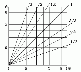
SLOPES ON LOG-LOG PAPER. It sometimes happens that the power value in an equation is known or assumed; the purpose of the graphical analysis is to find some other parameter of the equation. It is then justifiable to impose a straight line of the known slope onto the data points. It is easiest to construct lines of slope corresponding to integer powers or reciprocals of integers. Suppose you wanted a slope for power 2. Mark the point (n2,n) and connect it to the point (1,1) with a straight line. The number n can be any convenient value. Suppose we take n = 2. Then mark the points (4,2) and (1,1) and connect them with a straight line, which will have slope 2.

If you wanted the line corresponding to a power 3, you might take n = 2, then n³ = 8. So connect the points (8,2) and (1,1) with a straight line, which will have slope 3.

Fig. 7.13 shows this, for several different values of slope.