K-1 THE ACCELERATION DUE TO GRAVITY

Fig. 1. The Cenco apparatus.

1. PURPOSE

(1) To study uniformly accelerated motion in the case of a freely falling body.

(2) To test the hypothesis that the acceleration of a freely falling body is constant.

(3) To find the value of that constant, called the "acceleration due to gravity," g.

2. BACKGROUND

Read any textbook's treatment of kinematics and uniformly accelerated motion.

3. THE APPARATUS

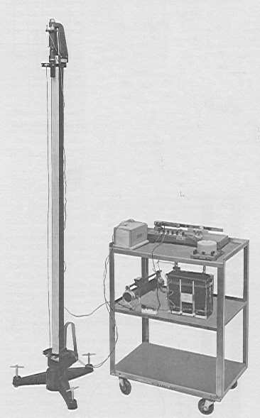
A steel plummet falls in a special apparatus which records its position as a function of time without disturbing its motion (Figs. 2 and 3). It falls along a 1.5 meter path between two parallel wires having a high electrical potential between them. A waxed paper tape lies along one of the wires. The potential of the wires alternates at a frequency of 60 Hz (derived from the building power lines). Sparks jump from one wire, to the plummet, through the waxed tape to the other wire, leaving a mark on the tape to mark the plummet's position. A spark occurs when the voltage is at or near its peak value, either positive or negative, so the spark rate is 120 Hz.

The clearance between the wires and the plummet must be small. The wires must therefore be exactly vertical to ensure that the plummet does not touch them on the way down. This adjustment is made with the leveling screws on the three feet of the apparatus and tested with a plumb bob.

The instructor will adjust the spark gap, and instruct you in the proper use of the apparatus, to avoid shocks. The voltage is high, but the current is low. Touching the wires won't kill you, but it doesn't feel good.

The plummet is initially held at the top of the apparatus by an electromagnet. The spark source is turned on first, then the magnet power is turned off. This releases the plummet, which falls and is caught in a felt lined (or sand filled) cup at the bottom. The spark source is then turned off before removing the waxed tape.

4. INTERPRETATION OF DATA

Fig. 2. The spark record on tape.

The waxed paper tape with the spark marks is the basis for all subsequent analysis. The spark marks at the beginning of the motion may be erratic and unreliable, so do not include them in the analysis. We do not need to know where the "zero" position was, for the analysis method uses only the changes in speed during the fall, that is, accelerations.

Table 1. A typical data record.
Spark Position 1 0.5 2 1.0 3 1.5 4 2.05 5 2.65 6 3.35 7 4.1 8 4.85 9 5.75 10 6.75 11 7.8 ......

Lay the data tape full length on the lab table, and tape it down at its ends (be careful not to stretch it.) Place a two-meter stick edge down on the tape so the stick markings lie as close to the spark marks as possible. Without moving the stick, record the position of every mark with respect to the stick. This is your data.

Write your name and your partner's name on the data tape. Carefully roll up the tape and secure it with a paper clip. Save it in case you should have to recheck your data. Do not hand it in with your report unless your instructor specifically requests it.

The data analysis methods described below use the following procedure: The marks on the tape represent position as a function of time. Compute the velocities during each time interval. If the acceleration is constant we expect these velocities to be a linear function of time. Therefore we have two tasks:

1. To determine whether the velocity-time relation is linear.

2. If it is linear, then compute the acceleration of the plummet.

While we usually encourage students to be creative and innovative in their approach to data collection and analysis, this experiment, simple as it seems, has some mathematical traps for the unwary. Even some laboratory manual authors have made the error of recommending invalid methods of data analysis. Therefore we urge the student to follow the following methods exactly as described.

5. METHOD 1. [All students will do this.]

The time interval between marks is 1/120 second. Since you will be making many calculations involving time intervals you can save yourself calculation drudgery by designating 1/120 second as the time "interval", the natural time "unit" for your selected points. The conversion from this unit to the more proper unit "second" can be made at the very end, when you calculate the final answers.

MARK    POSITION  VELOCITY
NO.     cm         cm/int

  1      0.5
                   0.5 
  2      1.0         
                   0.5
  3      1.5         
                   0.55
  4      2.05        
                   0.6
  5      2.65        
                   0.7
  6      3.35        
                   0.75
  7      4.1         
                   0.75
  8      4.85        
                   0.9
  9      5.75        
                   1.0
 10      6.75        
                   1.05
 11      7.8
                   1.1 
 12      8.9
                   1.65
 13     10.55
 - - - - - omitted data
 19     35.0
                   2.0
 20     37.0
                   2.2
 21     39.2

Table 2. Sample calculation sheet.

The data table might look something like the one in Table 2.

The numbers in this example show effects of indeterminate experimental errors.

The first column, "mark number" may also be interpreted as elapsed time, in the unit "interval."

The second data column has the positions of the spark marks. The velocities in the third column are computed average velocities in each "interval" of time. The velocities are obtained by subtracting successive entries in the position column.

Plot the average velocities (third column) against mark number (first column). This plot shows the change in velocity as a function of elapsed time. The velocities are "average" velocities during a time interval. As you will discover, the velocity-time relation is linear, so the average velocity occurs at the midpoint of the interval, and you can plot each point at the appropriate midpoint.

Is this plot a straight line? Should it be? If it is, find its slope in cm/interval2.

The slope of this line represents the acceleration, in the units (cm/interval)/interval = cm/(interval²) which is usually written cm-interval².

Choose two well-separated points on the ruler-drawn line. Use the line between these points as the hypotenuse of a right triangle whose legs are in the direction of the coordinate axes of the graph. The slope of the line is the quotient of the "lengths" of the legs of this triangle. [The "lengths" are not ruler-measured lengths, but are measured against the units of each graph axis. Therefore one "length" will be in the units "cm/interval," and the other will have the units "interval". These are time intervals.

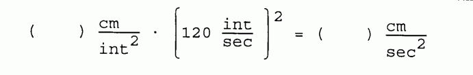
Convert this value of slope to the conventional units, cm/sec².

Since the unit "interval" is 1/120 sec, the conversion is done in this manner:

[1]

This average represents your final, "best" determination of the acceleration due to gravity, g. Is this answer reasonable?

What do you conclude, from these graphs, about the motion of the falling body?

The worksheet and summary of results which follow are for your convenience in laboratory. You will not hand in these pages, but will recopy and perhaps restructure this information in your report.

6. METHOD 2. [Instructor's option.]

The analysis method of section 5 made explicit use of a velocity-time graph. A strictly algebraic analysis is also possible. This avoids any additional error due to the errors in making the graph.

You should still include a velocity-time graph in your report to demonstrate that the acceleration really is constant. If it weren't, all of these methods for calculating the acceleration would be meaningless.

If the acceleration of the plummet is constant, it has the same value whatever time interval you choose, no matter whether the interval is large or small. The fractional error in each calculated acceleration is smaller if you choose larger intervals.

The best data analysis methods avoid combining or comparing calculations derived from the same data values. If the calculations use non-independent data values, subtle "cancellation" effects can occur. This method avoids that pitfall. [See the discussion of "successive differences" and "the method of differences" in section 8.2 of An Introduction to Experimental Analysis by Donald E. Simanek.]

[In the following paragraphs, "interval" refers to the number in column one of the data table, the intervals between your selected points.]

Since you have over forty calculated velocities, you can select independent pairs of them for acceleration calculations. You might choose interval no. 1 and 21, 2 and 22, 3 and 23 etc. spaced 20 time intervals apart. For example, the acceleration calculated using intervals 1 and 21 is

[2]

(2.3 cm/int - 0.5 cm/int)/(20 int) = 0.09 cm/int²

Do this for at least 20 pairs of intervals, to get 20 independent determinations of the acceleration. Average these accelerations. Convert the average to the units cm/sec² by Eq. (2) above.

7. METHOD 3. [Instructor's option.]

Group the position data into 16 or more equal time intervals Δt.

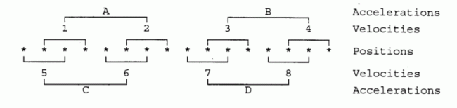Fig. 3. Data point grouping for method three.

Calculate velocities over the intervals labeled 1 through 8. These will have 2 Δt in the denominator, for the time interval is 2Δt. These velocities are clearly independent, for no two velocity calculations used the same position data points.

Now calculate four accelerations, labeled A through D in the diagram. They will all have 4Δt in the denominator. These accelerations are clearly independent. Average them. No position data has been used twice, so there is no possibility of data cancellation in the computation. From the point of view of error analysis, this method has the advantage of roughly equal weighting over the whole span of the data.

8. DISCUSSION OF RESULTS

(1) On the basis of your data, calculations and graphs can you say that the acceleration of the plummet was constant? Within what experimental error?

(2) Considering the "scatter" of the individual acceleration values, and the scatter of the points on the graphs, what error estimate (in %) would you give for your value of g?

(3) Compare your determination of g with that in the CRC handbook. Look up Helmert's equation in the handbook. You'll need to know that LHU is at 41° 8' North latitude, and the parking lot behind the physics labs is 580 feet above sea level. [You can check this data by consulting a U. S. Coast and Geodetic Survey map of the Lock Haven area.] This data, used in Helmert's equation, gives you the "accepted" value of g with which to compare yours. What is the percent discrepancy between your value and the accepted value?

9. QUESTIONS

(1) Suppose students at the University of Alaska did this experiment with the same apparatus. Would you expect them to obtain the same numeric result that you did? Be specific in explaining why or why not. What about students in the class of 2025 at Lunar Tech, doing this experiment on the moon with the same apparatus you used?

(2) Have you demonstrated the constancy of the acceleration due to gravity? No, you haven't, for it has different values in different places on earth! Have you demonstrated its constancy over time at this particular location? No, you demonstrated constancy only over a rather short time interval and within a certain range of uncertainty. You haven't demonstrated that it will have that value tomorrow! What have you demonstrated, in this experiment? Keep in mind that one should not claim more than is justified by the experiment.

(3) In this experiment the plummet was released from rest. A clever student wants to eliminate the closely spaced and unreliable sparks at the beginning of the tape. This student designs a plummet release mechanism which gives the plummet a downward push, only during a short interval before the beginning of the spark record. This makes the plummet velocity larger at the beginning of the spark tape. The student's lab partner worries that this might affect the experimental value of the acceleration due to gravity. What effect would it have on the calculated values of velocity? What effect would it have on the calculated value of g?

APPENDIX: USING A COMPUTER SPREADSHEET PROGRAM FOR ANALYSIS OF THE DATA

Any computer spreadsheet program is capable of performing the computations required in this experiment. We will illustrate the method with the Multiplan &tm; spreadsheet.

Spreadsheets structure data in rows and columns, just like the data sheets you make in lab. Each entry is called a "cell". The rows and columns are labeled, usually the columns have letter designations, the rows have number designations. We might speak of the cell C-5, which is the cell in the third column across the sheet and the fifth row down.

A cell may contain text or values. Cells with values may contain data or results. "Value" cells may contain mathematical formulae which specify how to calculate the value which will appear in the cell.

The spreadsheet you will use has the formulae already in place. On the screen it may look something like this:

ANALYSIS OF A FREELY FALLING BODY USING LEAST SQUARES FIT OF A STRAIGHT LINE Equation: y = mx + b Interval Position x (int) L (cm) y = dL/dx x^2 x*y 1 0.5 First data line 2 1 0.5 4 1 First reference line 3 1.5 0.5 9 1.5 4 2.05 0.55 16 2.2 5 2.65 0.6 25 3 6 3.35 0.7 36 4.2 7 4.1 0.75 49 5.25 8 4.85 0.75 64 6 9 5.75 0.9 81 8.1 10 6.75 1 100 10 ..... a large chunk of the spreadsheet has been omitted here ..... 60 141.15 4.3 3600 258 61 145.65 4.5 3721 274.5 62 150.1 4.45 3844 275.9 Last data line

x (int) L (cm) y x^2 x*y N --> 61 No. of points 1953 149.6 81374 6069.95 Summations Sum(x) Sum(y) Sum(x^2) Sum(x*y) N*Sum(x*y) 370266.95 Sumx*Sumy 292168.8 Numerator 78098.15 N*Sum(x^2) 4963814 (Sumx)^2 3814209 Denominator 1149605 Slope m 0.0679348 cm/int^2 g=m*(120^2) 978.26067 cm/sec^2 Accepted value 981 cm/sec^2 Abs. discrepancy -2.739328 Percent discrepancy -0.279238 % Intercept b 0.2774327 cm/int V at int 1= b * 120 33.291927 cm/sec True zero -b/m -4.083811 int

You will notice that this looks a lot like the data sheet you would make, though it shows far more decimal places than are significant.

This particular spreadsheet does not have the capability to show some math symbols. So it uses standard symbols used in computer programming:

^ raise to a power
* multiply

Column 1 contains a series of numbers labeling the sparks.

Column 2 contains the positions of each spark. These two columns contain all of the data; all other columns are the results of calculations on this data.

Column 3 contains the differences between entries in column 2. The formula in each cell of column 3 is the same: it takes the number in the same row, one column to the left, subtracts the number one column left and one row up, and enters the result. These are the "differences" y = dL/dx. (These are really ΔL and Δx, but this spreadsheet does not allow Greek letter symbols.)

The computer performs a linear regression analysis on the numbers in column 3. This gives the slope of the straight line which best fits the data. The process uses the squares of the y values, so a column is devoted to them. The products x*y are required also, and have their own column.

To enter your data you must first "blank" (erase) the data already in column 2. Do this by entering B (for "blank"). Put the cursor at the first entry of column 2 and enter a colon ":". Now move the cursor to the last data entry of column 2. (The "page down" key helps here.) The entries to be blanked are highlighted. When this is correct, press the "enter" key. Not only are the desired entries blanked, but any results calculated from them are also! Never fear, the necessary formulas are still intact, and will go to work as soon as you begin to enter data in column 2.

Do not delete any columns of this spreadsheet. You may wish to delete or add rows in the data area. But do not delete the rows labeled "First data line", "Last data line", or "Reference," since these contain formula references.

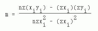
You should never use a tool without knowing how it works. The formulae being used here are the standard ones for linear regression where the errors are predominantly in one variable (y).

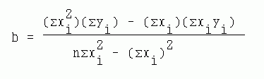
Let the data be y_i and x_i where i = 1, 2, ... n. We want to fit a straight line Y = mx + b to this data. (Upper case Y is used here, because values of Y_i obtained from the formula for the fitted curve will not in general be the same as the data points y_i). Then the slope (m) of the line and its y-intercept (b) are given by

[3,4]

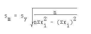
The standard deviation in the slope (s_m) and the standard deviationn of the y intercept (s_b) are:
[5,6]

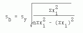The standard deviation of the y intercept is

[7,8]

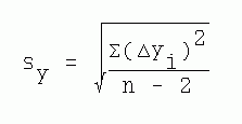Where s_y is the standard deviation of the individual data values from the fitted line. y_i represents the deviation of y_i from the fitted line and n is the number of data points.